The Nature of Radioactivity
Radioactivity can be referred to as a nuclear phenomenon. The combinations of neutrons and protons in the atom nucleus are different; they can be either stable or unstable. Therefore, certain combinations of protons and neutrons result in the unstable nature of the radioactive nucleus (People.chem.duke.edu. 2014). It causes redistributing the ratio between protons and neutrons aimed at obtaining the appropriate value of the existing stable nucleus. This type of redistribution leads to the emissions of peculiar radionuclide emanations that comprise radiations of the type alpha, bets and gamma. One of the most essential trait of the radioactive nucleus of some kind is the possibility of decay of an unstable nucleus in a certain period of time. Several repeated evaluations of counts from the sources of radioactivity per second do not provide the identical results; thus, the process of the radioactive decay is defined as statistical.
Radioactivity and its Statistical Nature
In case the number of measurements is considerable, it leads to the counts coming closer to the average value N. However, all the values will be either higher or lower than that distributed according to the principle: counts vs. frequency.
Experimental Procedure
1) A data set of 100“counts” can be generated via the use if the Excel function
(NORMSINV (RAND ())*SQRT (Your Student number)) + Your Student Number
2) The average of the set of counts is supposed to be close to your Student Number. A standard deviation is to be close to your student’s number square root.
3) The next step is calculating the standard and average deviations of the data sets.
4) The average data set is to be compared with the Student’s Number. The actual student number’s square root is to be compared with the data set of the standard deviation. The agreement of the values is to be explained thoroughly.
5) A histogram of the size of a full page is to be plotted with minimum 15 count intervals. The “count intervals in the X?axis and Number or occurrences or frequency on the “Y?Axis” are obligatory. The width of the histogram is to correspond with the one of the page, so the X?axis scale is to be expanded.
6) The set of data with normal distribution is to be compared with the expected one. A smooth curve is to be generated in the histogram.
7) The values demonstrated above in the step 3 and 4 are to be clearly shown.
8) With the help of the standard deviation, calculated on the basis of the data set and the histogram, one, two and three average deviations are to be shown graphically. Moreover, the percentage of the occurrences is to be calculated as well.
9) The next step is the comparison between the percentages of the occurrences with the values for one deviation predicted from a theoretical point of view (68%). The value is 96 % for the two deviations of standard type. Three standard deviations result in 99 %. The difference between the data set values and the theoretical knowledge is to be analyzed.
10) Analyze the possible result of taking 10 counts to undertake the stages 2-10. Discuss what would happen if 1,000 counts were applied.
11) Explain the relationship of the exercises with the radiation experiment management.
12) The results are to be compared with those of other students (two or more). The differences between the results are to be analyzed and discussed.
13) Background radiation plays an important role while taking actual measurements, in particular environmental samples. Explanations in brief are to be prepared.
Invite your friends and get bonus from each order they
have made!
· Observations with calculations
The observation of the completed experiment is taken and recorded. All the listed observations are available. Excel chart comprise 10, 100 and 1,000 samples with the additional plotted histogram. Presumably, the student’s number is 15135052.
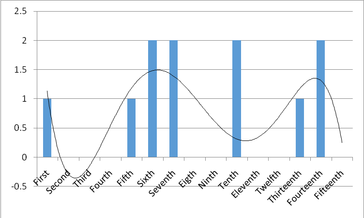
· A set of 10 counts are made using excel chart.

Figure 1: A 10-count chart
The calculations of the standard and average deviations are done on the basis of the data set. They are the following: average = 15135580, standard deviation = 5703.133027. My student’s number happened to be 15135052. I got the average of 15135580 on the basis of the data set. They are almost similar. The data set calculation enabled me to specify the square root of my student’s number = ?15135052= 3890; the value of the standard deviation (5703.133027) was obtained from the dataset calculation, it is close.
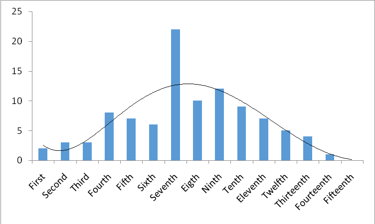
· A 100-count data set made using excel chart.

Figure 2: A 100-count chart
The calculations of the standard and average deviations are done on the basis of the data set. They are the following: average = 15135071, standard deviation = 3936.940991. My student’s number happened to be 15135052. I got the average of 15135071 on the basis of the data set. They are almost similar. The data set calculation enabled me to specify the square root of my student’s number = ?15135052 = 3890; the value of the standard deviation (3936.940991) was obtained from the dataset calculation, it is close.
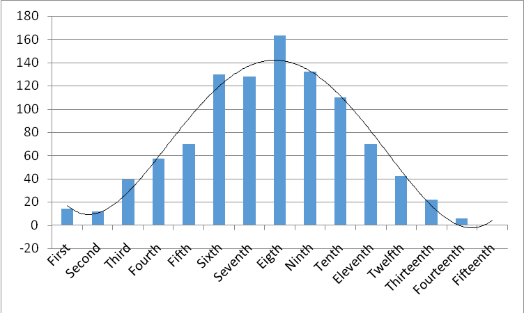
· A 1,000 count set made using excel chart.

Figure 3: A 1000-count chart
The calculations of the standard and average deviations are done on the basis of the data set. They are the following: average = 15134820, standard deviation = 3981.203056. My student’s number happened to be 15135052. I got the average of 15134820 on the basis of the data set. They are almost similar. The data set calculation enabled me to specify the square root of my student’s number = ?15135052 = 3890; the value of the standard deviation (3981.203056) was obtained from the dataset calculation, it is close.
4) Compare the data set AVERAGE with your student number and the data set
STANDARD DEVIATION with the actual square root of your student’s number. Do the values agree and if not comment of why not?
The radioactive decay is characterized as a statistical process. The number of counts can vary for various types of measurements. So, the values do not agree (Physics.org. 2014). A particular characteristic of a certain radionuclide is high possibility of decay of the unstable nucleus in a certain period of time. Repeating the counting we cannot expect getting the same outputs.
9) The percentage of occurrences is to be compared with the percentage of the predicted values in theory. One standard deviation has the predicted value of 68%. It is 96% for the two-standard deviation, while for three-standard deviation it is 99%. There are certain differences between the values of data sets and the theoretical measurements.
| No of samples | |
|
|
| 10 | 3229.465 | 10.429.444 | 15135052/10429444=1.45 |
| 100 | 3959.16 | 150674.948 | 15135052/15674948=0.96 |
| 1000 | 3981.2 | 15.849.953 | 15135052/15849953=0.95 |
The above mentioned values in the table are approved for the curves which show 10, 100 and 1000 samples respectively. A wide curve with two peaks is possible if n = 10. In this case, it demonstrated dispersion of the counts. A normal distribution chart with the curve and mostly central concentration of the data stipulates for n = 10, n=1,000. The endorsement rate of the values is 95 and 96 % respectively.
10) Discuss what would happen if a set of 1000 counts were used on undertaking steps 2 to 10? What would happen if only 10 counts were taken?
The increase in the count number, there is a move of the distribution diagram to the central area. The diagram also gets wider. A normal distribution chart that is wide and symmetrical requires the high value of 1,000. The area of the band of 3? comprises approximately 98 % of counts or even more. Large deviations and scattering of the chart are the results of using 10 counts. It causes an opposite effect.
11) All the experiments concerning radiation are managed in the way which is related to the mentioned exercises. Data could be controlled more effectively, if there is less uncertainty and exact figures and numbers are applied with proper intervals, numbers and samples.
13) In making real measurements, especially of environmental samples, background radiation can play a significant role in the final outcome of any final measurement and its uncertainty. Briefly describe what that might be.
Taking into consideration assessing the count rate being not far from the source of radiation, the measurement of the Geiger counter is done to evaluate the total rate in the background and the source (Fireworld.com 2014). The measurement is not very reliable owing to that. This uncertainty is only increased; though, it is possible to eliminate the background effect. It is necessary to measure the background late (even if it is extremely low) to be able to perform the real rate measurement with the calculated background rate effect. Such methods as measuring the rate which remains or displacement of the source of radioactivity along with others are applied.
Struggling with your essay?
Ask professionals to help you!
Start Chat
Conclusion
The present experiment comprised plotting the histogram, making observations and studying the new phenomena. It was conducted in strict accordance with the objectives. The theoretical values of Standard Deviation and Average were contrasted with the values calculated independently. High uncertainty of distribution and scattered character of data were peculiar to the cases of n=10, i.e. the low number of samples. The increase in the number of samples caused decrease in spreading the data, a smooth curve, and the appearance of a good distribution chart (Saha 2006, 34). Almost total similarity (about 95%) between the theoretical data and practical knowledge is found for the values of n equal to 100 and 1,000. It can be explained through a great number of used samples. If more than thirty samples are taken for the distribution model of Poisson, it is a high number (Umass.edu. 2014).


